Thinking it doesn't make any sense that BIO_13 precipitation of the warmest month is most important. I also included BIO_18 precipitation of the warmest quarter.

Due to correlation values, you have to make a decision when the going gets rough. I am now going to include BIO_12 [Annual Precipitation], keep 16, get rid of 13 and 14.

R script:
#load packages
library(raster)
library(maptools)
library(dismo)
library(rJava) #also make sure to put maxent.jar into R dismo library folder

#convert to raster
altitude<-raster("/Volumes/LOLOYOHE BA/Merged_layers/alt_seasia9tile.grd")
bio2<-raster("/Volumes/LOLOYOHE BA/Merged_layers/bio2_seasia9tile.grd")

bio2<-raster("/Volumes/LOLOYOHE BA/Merged_layers/bio2_seasia9tile.grd")
bio5<-raster("/Volumes/LOLOYOHE BA/Merged_layers/bio5_seasia9tile.grd")
bio8<-raster("/Volumes/LOLOYOHE BA/Merged_layers/bio8_seasia9tile.grd")
bio12<-raster("/Volumes/LOLOYOHE BA/Merged_layers/bio12_seasia9tile.grd")
bio15<-raster("/Volumes/LOLOYOHE BA/Merged_layers/bio15_seasia9tile.grd")
bio16<-raster("/Volumes/LOLOYOHE BA/Merged_layers/bio16_seasia9tile.grd")
bio18<-raster("/Volumes/LOLOYOHE BA/Merged_layers/bio18_seasia9tile.grd")
bio19<-raster("/Volumes/LOLOYOHE BA/Merged_layers/bio19_seasia9tile.grd")


#stack the layers into one raster and name the layers within the stack

stacked.layers<-stack(altitude, bio2, bio5, bio8, bio12, bio15, bio16, bio18, bio19)
names(stacked.layers)<-c("altitude", "bio2", "bio5", "bio8", "bio12", "bio15", "bio16", "bio18", "bio19")
#remove the original rasters for space
rm(altitude, bio2, bio5, bio8, bio12, bio15, bio16, bio18, bio19)

#read locality points for first species: alcippe peracensis

peracensis.pts<-readShapePoints("/Volumes/LOLOYOHE BA/Vietnam Data/maxent_models/alcippe_peracensis_all.shp")

#run maxent for first species
maxent.peracensis<-maxent(stacked.layers, coordinates(peracensist.pts)[,1:2])

#see graph of important variables

plot(maxent.peracensis)

#see the response curves
response(maxent.peracensis)

#make raster from predictions
r.peracensis<-predict(maxent.peracensis, stacked.layers, progress = "window")


These are my models for six species showing differences between before and after changing the BIOCLIM variables to include. Notice the before is run using the maxent.jar applet rather than with R so I am still figuring out how to get all the same outputs

Alcippe peracensis Mountain fulvetta
Before:

Variable	Percent contribution	Permutation importance
bio13_seasia9tile	61.1	61.4
bio14_seasia9tile	18.1	4.3
bio15_seasia9tile	9.4	28.4
_alt_seasia9tile	7.4	0.7
_bio2_seasia9tile	3.3	1.3
bio8_seasia9tile	0.6	2
_bio5_seasia9tile	0.2	1.9

After:

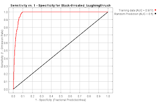
Garrulax chinensis Black-throated laughingthrush

Before:

Variable	Percent contribution	Permutation importance
bio13_seasia9tile	53.7	52.6
bio15_seasia9tile	25.7	18.2
bio14_seasia9tile	6	4.3
bio8_seasia9tile	5.5	1
_bio2_seasia9tile	4	1.3
_bio5_seasia9tile	3.9	17.4
_alt_seasia9tile	1.1	5.2

After:

Garrulax leucolophus White-crested laughingthrush

Before: 

Variable	Percent contribution	Permutation importance
bio13_seasia9tile	58.6	29.3
_bio5_seasia9tile	11.3	6.5
_alt_seasia9tile	9	18.8
_bio2_seasia9tile	7.6	13.1
bio14_seasia9tile	5.5	7.1
bio15_seasia9tile	5.1	1.5
bio8_seasia9tile	2.9	23.7

After:

Pellorneum albiventre Spot-throated babbler
Before:

Variable	Percent contribution	Permutation importance
bio13_seasia9tile	57.5	74.3
_alt_seasia9tile	17.4	1.9
bio15_seasia9tile	12.9	6.5
bio14_seasia9tile	11.8	16.9
_bio2_seasia9tile	0.2	0.5
_bio5_seasia9tile	0.1	0
bio8_seasia9tile	0	0

After:

Pomatorhinus ruficollis Streak-breasted scimitar babbler
Before:

Variable	Percent contribution	Permutation importance
bio13_seasia9tile	58.6	29.3
_bio5_seasia9tile	11.3	6.5
_alt_seasia9tile	9	18.8
_bio2_seasia9tile	7.6	13.1
bio14_seasia9tile	5.5	7.1
bio15_seasia9tile	5.1	1.5
bio8_seasia9tile	2.9	23.7

After:

Pteruthius

Should I even bother including in my analysis anymore? (No longer a babbler)

Questions to discuss:

1. Is it okay to rerun models with new set of BIOCLIM variables even if you have already run it once and just notice the first one does not seem biologically true? What if these new variables don't seem right either? Is it okay to keep trying to rerun the models?
2. What does it mean when only one variable is giving strong response?
3. Precipitation of the Wettest Month (BIO13) was removed as we had thought this didn't make much biological sense due to the way the rainy season works in SE Asia (May/June-Sept/October). We thought it made more sense if Precipitation of the Wettest Quarter were included instead (BIO 16). However, this only seemed to be important for P. ruficollis (as well as altitude). Annual precipitation seemed to be the only important variable (BIO 12) for all other species and nothing else. How can we interpret this?
4. How do I make the ROC curve in R?
5. I want to validate the model and move forward from this.

First PCR as a PhD student. Sigh.

PCR#:	LY0001
	30 μL reaction
		# Tubes:	8
MasterMix	Single Tube (μL)	Total in MM (μL)
Buffer	3	24
MgCl2	3	24
dNTPs	0.5	4
Taq	0.5	4
H20	13	104
FW	3	24
RV	3	24
DNA	4	X
FW Primer	THYF
RV Primer	THYR
Tube#	Sample
1	588460
2	580656
3	110278
4	108297
5	560781
6	control
Program:	Omar1
Annealing Temp:	50

Sample #s correlate with AMCC AMNH tissue number.

Created 9 tile layer of all the BIOCLIM and altitude. The only way I could figure out how to do it was in DIVA-GIS (although I am sure there is a (much faster!) way to do it in R).

• Downloaded tiles 18, 19, 110, 28, 29, 210, 38, 39, 310.
• Import each file to DIVA-GIS and convert all to .grd files.
• Grid-->Merge and merge tiles but can only do 2 at a time. 
• Finally will have a merged tile that is 60W-150W; -30S-60N

Finally, figured out how to correlate the BIOCLIM variables using R.

• Upload all 19 layers plus altitude into R using the "raster" package.
  Rcommand:
  
  >bioclim1<-raster("/VOLUMES/LOLOYOHE BA/ Merged_layers/bio1_seasia9tile.grd")
  ...
  >bioclim19<-raster("/VOLUMES/LOLOYOHE BA/ Merged_layers/bio19_seasia9tile.grd")
  #stack the rasters
  >rastStack <- stack (altitude, bioclim1, bioclim2 ... bioclim19)
  >install.packages("dismo")
  >require(dismo)
  >pairs (rastStack, hist=TRUE, cor=TRUE, use="pairwise.complete.obs", maxpixels=10000)
• Using the correlation matrix, I made my figure for the supplementary material for the manuscript.
• Layers to include in analysis: altitude, BIO_2, BIO_5, BIO_8, BIO_13, BIO_14, BIO_15, BIO_18, BIO_19

Installing compiler on mac (for the millionth time!!)
http://www.mkyong.com/mac/how-to-install-gcc-compiler-on-mac-os-x/

To install DIVA-GIS
-Installed WineBottler
-To get WineBottler to work--had to install wget command: http://www.mactricksandtips.com/2008/07/installing-wget-on-your-mac-for-terminal.html
-WineBottler was missing WineTricks to install missing libraries with DIVA-GIS: http://code.google.com/p/winetricks/wiki/Installing
NEVERMIND--gave up on this. Could never figure out how to install the two missing libraries in winetricks in order for WineBottler to run properly.
--ended up installing DIVA-GIS on PC for now.

Setting up data for DIVA-GIS and maxent
http://www.bioversityinternational.org/fileadmin/bioversity/publications/pdfs/1431_Training_manual_on_spatial_analysis_of_plant_diversity_and_distribution.final.pdf

------------------------------------------
Running this in R.

Import data point

file name: "C:/PROGRA~1/R/R-211~1.1/library/dismo/ex/garrulax_chinensis_all.csv"

#plot map of SE asia
plot(wrld_simpl, xlim=c(80-110), ylim=c(-20,30) axes=TRUE,col='light yellow')


------------------------------------------
What I want my paper to be like:
http://www.plosone.org/article/info%3Adoi%2F10.1371%2Fjournal.pone.0009612
and maybe this:
http://phylodiversity.net/fslik/index_files/BiolCon2012.pdf

Notes on Simpson's Tempo and Mode in Evolution

Chapter II: Determinants of Evolution (p. 93-96)

• Variability: 
• High variability in groups is usually a result of other factors
• Can lead to rapid differentiation on low taxonomic levels but cannot be responsible for creating new high taxonomic levels
• Cannot be responsible for moderate-high rates of evolution
• Most lineages show a constant variability over evolutionary time and a rapid deviation to increase variability
• Maximum rates of evolution usually have low rather than high variability
• Rate of mutation: mutation necessary for evolution to occur
• Mutation rate NOT same as rate of evolution
• Character of mutation
• Single mutations with large, discrete phenotypic effects usually unimportant in evolution
• Saltation (large step change) could arise from practically impossible genetic scenarios
• Mutations recognizable in sequence usually have no/little phenotypic effect
• Many small mutations consistent with high rates of evolution--small fluctuations in developmental fields
• Length of generation
• Temporal rate of evolution should vary inversely with generation time
• May influence unusually high rates of evolution
• Population Size
• Large populations: evolution is extremely slow under selection and evolution is proportional to selection intensity--tend to be at genetic equilibrium even though more variable which is not good for rapid evolution
• Small populations: more susceptible to drift--maximum rates of evolution seen in small populations but it is nonadaptive and most likely lead to extinction or rare adaptive reorientation
• Selection: has direction and intensity--crucial factor for evolution but may be ineffective at times
• Direction can either be centripetal (concentrate population to single modal type), centrifugal (diverge population), or linear (shift modal type to one position or another). 

Chapter III: Micro-evolution, macro-evolution, and mega-evolution (p. 97-124)

• Investigates the question of saltations and their likelihood
• Discusses many discontinuities in fossil record
• Mega-evolution normally evolves among small populations that become pre-adaptive and evolve continuously to different ecological conditions
• Large population fragments and new mutations randomly fix (rarely preadaptive)

Chapter IV: Low rate and high rate lines (p. 147-148)

• Bradytely: slower than standard
• Not dependent on mutation rate
• Usually result from rapid evolution--not necessarily primitive
• Characters are predominantly adaptive
• Horotely: standard rate of evolution for an organism
• Trachytely: faster than standard--either become extinct or have massive adaptive 
• More recent rapidly evolving groups more vulnerable to extinction
• Less specialized bradytely survive longer than more specialized

Chapter V: Inertia, Trend, and Momentum (p. 177-179)

• Orthogenesis (rectilinear evolution): tendency for phyla to continue to evolve in same direction for considerable periods of time [only descriptive statement]
• Typical of large populations evolving at moderate rates
• Not simple, linear, unbranched evolution--can have many changes in rates throughout time 
• Most linearity due to heredity
• Direction of mutation doesn't really have anything to do with direction of evolution
• Response to selection is not instantaneous, and inertia (lage in following a shifting optimum), is an important element in evolution

Chapter VI: Organism and Environment (p. 181-196)

• Adaptive zone: organism's environment and everything involved in the situation in which the organism is an element
• Can evolve!

Chapter VII: Modes of Evolution (p. 216-217)

• Speciation: local differentiation of two or more groups within a more widespread population
• Low taxonomic level
• Local adaptation and random segregation
• Phyletic evolution: sustained, directional shift of the average characters of populations
• Post adaptation-- little random change
• Quantum evolution: relatively rapid shift of biotic population in disequilibrium to an equilibrium distinctly unlike an ancestral condition
• High taxonomic level
• Preadaptation (usually preceded by inadaptive change)

Yay, I finished a book :)

Ran MAXENT for 6 species (see file Babblers_AllMuseumDistribution.xlsx):
G. leucolophus, G. chinensis, A. peracensis, P. albiventre, P. ruficollis, and P. flaviscapis

1) Convert .xls file to .csv file with three columns for each species--species name, longitude, latitude

2) Add .csv file to MAXENT

3) Also add 19 BIOCLIM variables. Need to figure out how I had put them in the correct format--something to do with DIVA-GIS.

Output was interesting results. Probably meaningless until BIOCLIM variables are correlated.

Tomorrow (Thursday, 10 Jan):

• Correlate the BIOCLIM variables and rerun MAXENT
• Load layers into qGIS
• Download and add land use data

Notes on Simpson's Tempo and Mode in Evolution:

• Tempo: evolutionary rates under natural conditions, the measurement and interpretation of rates, their acceleration and deceleration, the conditions of exceptionally slow or rapid evolutions, and phenomena suggestive of inertia and momentum. (p. xxix)
• Mode: study of the way, manner, or pattern of evolution, how populations become genetically and morphologically differentiated, and how they have passed from one way of living to another or failed to do so. (p. xxx)

Chapter I: Rates of evolution

• Four basic theorems concerning rates of evolution (p. 12)
• Rate of evolution of one character may be a function of another character and not genetically separable even though the rates are not equal
• Rate of evolution of any character or combination of characters may change markedly at any time in phyletic evolution, even though the direction of evolution remains the same. 
• Rates of evolution of two or more characters within a single phylum may change independently 
• Two phyla of common ancestry may become differentiated by different rates of evolution of different characters, without any marked qualitative differences or differences in direction of evolution
• Need to come up with a way to not only think in terms of unit characters--might be better to think of the organism as a whole