Finally have some meaningful(?) output. This is going to be lengthy but it will be really helpful in organizing my thought. Because I had been including morphological data for very "distantly-related babblers", all of the nodes for the rate shifts occurred, of course on the root node. I removed some more taxa to only include measurements for birds within the babbler family. Therefore, I reran the PCA. Still similar trends:

Count the number of species in my analysis and the number of specimens per species.
> babblers.species.count<-ddply(.data=new.babblers, .(Genus, Species), species.count=length(Wing.Length), summarize)
> babblers.species.count
Genus Species species.count
1 Actinodura egertoni 6
2 Actinodura morrisoniana 3
3 Actinodura nipalensis 3
4 Actinodura waldeni 5
5 Alcippe brunneicauda 4
6 Alcippe grotei 11
7 Alcippe morrisonia 5
8 Alcippe peracensis 2
9 Alcippe poioicephala 11
10 Babax lanceolatus 4
11 Cutia nipalensis 7
12 Dumetia hyperythra 6
13 Gampsorhynchus rufulus 8
14 Garrulax affinis 11
15 Garrulax albogularis 5
16 Garrulax canorus 14
17 Garrulax chinensis 40
18 Garrulax cineraceus 4
19 Garrulax erythrocephalus 1
20 Garrulax formosus 4
21 Garrulax leucolophus 41
22 Garrulax lineatus 6
23 Garrulax maesi 3
24 Garrulax merulinus 1
25 Garrulax milleti 1
26 Garrulax milnei 4
27 Garrulax mitratus 6
28 Garrulax monileger 8
29 Garrulax nuchalis 3
30 Garrulax ocellatus 7
31 Garrulax palliatus 4
32 Garrulax poecilorhynchus 4
33 Garrulax sannio 12
34 Garrulax squamatus 3
35 Garrulax striatus 6
36 Garrulax subunicolor 6
37 Garrulax variegatum 3
38 Garrulax virgatus 2
39 Heterophasia auricularis 3
40 Heterophasia capistrata 6
41 Heterophasia gracilis 4
42 Heterophasia maelanoleuca 9
43 Heterophasia picaoides 7
44 Heterophasia pulchella 3
45 Illadopsis albipectus 4
46 Illadopsis cleaveri 4
47 Illadopsis fulvescens 8
48 Illadopsis puveli 2
49 Illadopsis pyrrhoptera 2
50 Illadopsis rufescens 3
51 Illadopsis rufipennis 6
52 Kenopia striata 2
53 Leiothrix argentauris 15
54 Leiothrix lutea 4
55 Liocichla phoenicea 1
56 Liocichla steeri 3
57 Macronus gularis 25
58 Macronus ptilosus 3
59 Macronus striaticeps 12
60 Malacocincla abbotti 4
61 Malacocincla cinereiceps 2
62 Malacocincla malaccensis 6
63 Malacocincla sepiaria 3
64 Malacopteron affine 3
65 Malacopteron albogulare 4
66 Malacopteron cinereum 1
67 Malacopteron magnirostre 7
68 Malacopteron magnum 5
69 Malacopteron palawanenese 3
70 Minla ignotincta 6
71 Minla strigula 7
72 Napothera brevicaudata 4
73 Napothera crassa 2
74 Napothera crispifrons 7
75 Napothera epilepidota 10
76 Pellorneum albiventre 9
77 Pellorneum capristratum 15
78 Pellorneum pyrrogenys 6
79 Pellorneum ruficeps 5
80 Pellorneum tickelli 1
81 Phyllanthus atripennis 6
82 Pomatorhinus erythrogenys 18
83 Pomatorhinus ferruginosus 4
84 Pomatorhinus horsfieldi 6
85 Pomatorhinus hypoleucos 4
86 Pomatorhinus montanus 4
87 Pomatorhinus ruficollis 9
88 Pomatorhinus swinhoei 2
89 Ptilocichla falcata 2
90 Ptilocichla leucogrammica 3
91 Ptilocichla mindanensis 3
92 Ptyrticus turdinus 6
93 Rhopocichla atriceps 4
94 Rimator malacoptilus 3
95 Schoeniparus brunnea 10
96 Schoeniparus castaneceps 1
97 Schoeniparus cinerea 3
98 Schoeniparus dubia 6
99 Schoeniparus rufogularis 9
100 Spelaeornis chocolatinus 5
101 Spelaeornis troglodytoide 3
102 Sphenocichla humei 3
103 Stachyris ambigua 4
104 Stachyris chrysaea 11
105 Stachyris erythroptera 8
106 Stachyris grammiceps 2
107 Stachyris leucotis 3
108 Stachyris maculata 3
109 Stachyris melanothorax 6
110 Stachyris nigriceps 7
111 Stachyris nigricollis 4
112 Stachyris oglei 3
113 Stachyris poliocephala 4
114 Stachyris pyrrhops 3
115 Stachyris ruficeps 10
116 Stachyris rufifrons 3
117 Stachyris striolata 5
118 Stachyris thoracica 4
119 Timalia pileata 8
120 Trichastoma bicolor 4
121 Trichastoma celebense 11
122 Trichastoma rostratum 5
123 Turdoides bicolor 3
124 Turdoides gularis 4
125 Turdoides jardineii 10
126 Turdoides plebejus 16
127 Turdoides reinwardii 3
128 Xiphirhynchus superciliaris 3
I had to match up the names of my species with the names on the tips (huge pain) and I ended up doing it by hand--I could have probably scripted it but I think it would have taken me just as long.
I collapsed the PCA values into means for each species but I believe I already posted the script for that. So now I have a .csv that contains all the mean PCA that corresponds to each species with the species name that matches the tip. YAY.
Now I finally have evol.rate.mcmc() running and I ran the output for the first four principle components:
#read in the PCA vector:
temp<-read.csv(file.choose())
x<-as.vector(temp$Tarsus) #vector of tarsus measurement traits
names(x)<-as.vector(temp$Species) #names the measurements
#i have to date the trees
undated.tree<-read.tree(file.choose())
#the tree was based on two calibration points (see Moyle, et al. 2012) and the root
tree<-chronopl(undated.tree, lambda=.5, age.min=c(8.4, 13, 27.1), age.max=c(11.4,17, 37.3), node = c(336, 297, 293))
#now time for the juicy part--using default parameters to start with as suggested by Revell, et al. 2011
result<-evol.rate.mcmc(tree,x,ngen=100000,control=list(sd2=2.0,sdlnr=3.0))
min_split<-minSplit(tree,result$mcmc[21:101,c("node","bp")])
mcmc<-posterior.evolrate(tree,min_split,result$mcmc[21:101,],result$tips[201:1001])
mcmc.data.1<-as.data.frame(mcmc)
#nicely summarize the mcmc for Tarsus
output.summary.1<-ddply(.data=mcmc.data.1, .(node), node.count=length(bp), mean.bp=mean(bp),mean.sig1=mean(sig1), mean.sig2=mean(sig2), summarize)

#let's visualize the nodes! first trim the tree to visualize only nodes that were used in analysis
trim.tree<-drop.tip(tree,tree$tip.label[-(match(names(x),tree$tip.label))])
Nodes 3 and 4 are probably root nodes and have high probability. Let's look at 186, 185, and 188.
#now extract the clades we want to look at
this.extract<-extract.clade(tree.trim, tree.trim$edge[186])


temp<-read.csv(file.choose())
x<-as.vector(temp$Bill.Length) #vector of bill length measurement traits
#you have to reset the names
names(x)<-as.vector(temp$Species) #names the measurements
#use the same dated tree as before
result<-evol.rate.mcmc(tree,x,ngen=100000,control=list(sd2=2.0,sdlnr=3.0))
min_split<-minSplit(tree,result$mcmc[21:101,c("node","bp")])
mcmc<-posterior.evolrate(tree,min_split,result$mcmc[21:101,],result$tips[201:1001])
mcmc.data.2<-as.data.frame(mcmc)
#nicely summarize the mcmc for Bill Length
output.summary.2<-ddply(.data=mcmc.data.2, .(node), node.count=length(bp), mean.bp=mean(bp),mean.sig1=mean(sig1), mean.sig2=mean(sig2), summarize)

#you have to reset the names
names(x)<-as.vector(temp$Species) #names the measurements
#use the same dated tree as before
result<-evol.rate.mcmc(tree,x,ngen=100000,control=list(sd2=2.0,sdlnr=3.0))
min_split<-minSplit(tree,result$mcmc[21:101,c("node","bp")])
mcmc<-posterior.evolrate(tree,min_split,result$mcmc[21:101,],result$tips[201:1001])
mcmc.data.2<-as.data.frame(mcmc)
#nicely summarize the mcmc for hallux
output.summary.2<-ddply(.data=mcmc.data.3, .(node), node.count=length(bp), mean.bp=mean(bp),mean.sig1=mean(sig1), mean.sig2=mean(sig2), summarize)
 Node 9 has high probability (low frequency):
> this.extract<-extract.clade(tree.trim, tree.trim$edge[9])
> plot(this.extract)


#you have to reset the names
names(x)<-as.vector(temp$Species) #names the measurements
#use the same dated tree as before
result<-evol.rate.mcmc(tree,x,ngen=100000,control=list(sd2=2.0,sdlnr=3.0))
min_split<-minSplit(tree,result$mcmc[21:101,c("node","bp")])
mcmc<-posterior.evolrate(tree,min_split,result$mcmc[21:101,],result$tips[201:1001])
mcmc.data.2<-as.data.frame(mcmc)
#nicely summarize the mcmc for tail length
output.summary.4<-ddply(.data=mcmc.data.4, .(node), node.count=length(bp), mean.bp=mean(bp),mean.sig1=mean(sig1), mean.sig2=mean(sig2), summarize)


Count the number of species in my analysis and the number of specimens per species.
> babblers.species.count<-ddply(.data=new.babblers, .(Genus, Species), species.count=length(Wing.Length), summarize)
> babblers.species.count
Genus Species species.count
1 Actinodura egertoni 6
2 Actinodura morrisoniana 3
3 Actinodura nipalensis 3
4 Actinodura waldeni 5
5 Alcippe brunneicauda 4
6 Alcippe grotei 11
7 Alcippe morrisonia 5
8 Alcippe peracensis 2
9 Alcippe poioicephala 11
10 Babax lanceolatus 4
11 Cutia nipalensis 7
12 Dumetia hyperythra 6
13 Gampsorhynchus rufulus 8
14 Garrulax affinis 11
15 Garrulax albogularis 5
16 Garrulax canorus 14
17 Garrulax chinensis 40
18 Garrulax cineraceus 4
19 Garrulax erythrocephalus 1
20 Garrulax formosus 4
21 Garrulax leucolophus 41
22 Garrulax lineatus 6
23 Garrulax maesi 3
24 Garrulax merulinus 1
25 Garrulax milleti 1
26 Garrulax milnei 4
27 Garrulax mitratus 6
28 Garrulax monileger 8
29 Garrulax nuchalis 3
30 Garrulax ocellatus 7
31 Garrulax palliatus 4
32 Garrulax poecilorhynchus 4
33 Garrulax sannio 12
34 Garrulax squamatus 3
35 Garrulax striatus 6
36 Garrulax subunicolor 6
37 Garrulax variegatum 3
38 Garrulax virgatus 2
39 Heterophasia auricularis 3
40 Heterophasia capistrata 6
41 Heterophasia gracilis 4
42 Heterophasia maelanoleuca 9
43 Heterophasia picaoides 7
44 Heterophasia pulchella 3
45 Illadopsis albipectus 4
46 Illadopsis cleaveri 4
47 Illadopsis fulvescens 8
48 Illadopsis puveli 2
49 Illadopsis pyrrhoptera 2
50 Illadopsis rufescens 3
51 Illadopsis rufipennis 6
52 Kenopia striata 2
53 Leiothrix argentauris 15
54 Leiothrix lutea 4
55 Liocichla phoenicea 1
56 Liocichla steeri 3
57 Macronus gularis 25
58 Macronus ptilosus 3
59 Macronus striaticeps 12
60 Malacocincla abbotti 4
61 Malacocincla cinereiceps 2
62 Malacocincla malaccensis 6
63 Malacocincla sepiaria 3
64 Malacopteron affine 3
65 Malacopteron albogulare 4
66 Malacopteron cinereum 1
67 Malacopteron magnirostre 7
68 Malacopteron magnum 5
69 Malacopteron palawanenese 3
70 Minla ignotincta 6
71 Minla strigula 7
72 Napothera brevicaudata 4
73 Napothera crassa 2
74 Napothera crispifrons 7
75 Napothera epilepidota 10
76 Pellorneum albiventre 9
77 Pellorneum capristratum 15
78 Pellorneum pyrrogenys 6
79 Pellorneum ruficeps 5
80 Pellorneum tickelli 1
81 Phyllanthus atripennis 6
82 Pomatorhinus erythrogenys 18
83 Pomatorhinus ferruginosus 4
84 Pomatorhinus horsfieldi 6
85 Pomatorhinus hypoleucos 4
86 Pomatorhinus montanus 4
87 Pomatorhinus ruficollis 9
88 Pomatorhinus swinhoei 2
89 Ptilocichla falcata 2
90 Ptilocichla leucogrammica 3
91 Ptilocichla mindanensis 3
92 Ptyrticus turdinus 6
93 Rhopocichla atriceps 4
94 Rimator malacoptilus 3
95 Schoeniparus brunnea 10
96 Schoeniparus castaneceps 1
97 Schoeniparus cinerea 3
98 Schoeniparus dubia 6
99 Schoeniparus rufogularis 9
100 Spelaeornis chocolatinus 5
101 Spelaeornis troglodytoide 3
102 Sphenocichla humei 3
103 Stachyris ambigua 4
104 Stachyris chrysaea 11
105 Stachyris erythroptera 8
106 Stachyris grammiceps 2
107 Stachyris leucotis 3
108 Stachyris maculata 3
109 Stachyris melanothorax 6
110 Stachyris nigriceps 7
111 Stachyris nigricollis 4
112 Stachyris oglei 3
113 Stachyris poliocephala 4
114 Stachyris pyrrhops 3
115 Stachyris ruficeps 10
116 Stachyris rufifrons 3
117 Stachyris striolata 5
118 Stachyris thoracica 4
119 Timalia pileata 8
120 Trichastoma bicolor 4
121 Trichastoma celebense 11
122 Trichastoma rostratum 5
123 Turdoides bicolor 3
124 Turdoides gularis 4
125 Turdoides jardineii 10
126 Turdoides plebejus 16
127 Turdoides reinwardii 3
128 Xiphirhynchus superciliaris 3
I had to match up the names of my species with the names on the tips (huge pain) and I ended up doing it by hand--I could have probably scripted it but I think it would have taken me just as long.
I collapsed the PCA values into means for each species but I believe I already posted the script for that. So now I have a .csv that contains all the mean PCA that corresponds to each species with the species name that matches the tip. YAY.
Now I finally have evol.rate.mcmc() running and I ran the output for the first four principle components:
#read in the PCA vector:
temp<-read.csv(file.choose())
x<-as.vector(temp$Tarsus) #vector of tarsus measurement traits
names(x)<-as.vector(temp$Species) #names the measurements
#i have to date the trees
undated.tree<-read.tree(file.choose())
#the tree was based on two calibration points (see Moyle, et al. 2012) and the root
tree<-chronopl(undated.tree, lambda=.5, age.min=c(8.4, 13, 27.1), age.max=c(11.4,17, 37.3), node = c(336, 297, 293))
#now time for the juicy part--using default parameters to start with as suggested by Revell, et al. 2011
result<-evol.rate.mcmc(tree,x,ngen=100000,control=list(sd2=2.0,sdlnr=3.0))
min_split<-minSplit(tree,result$mcmc[21:101,c("node","bp")])
mcmc<-posterior.evolrate(tree,min_split,result$mcmc[21:101,],result$tips[201:1001])
mcmc.data.1<-as.data.frame(mcmc)
#nicely summarize the mcmc for Tarsus
output.summary.1<-ddply(.data=mcmc.data.1, .(node), node.count=length(bp), mean.bp=mean(bp),mean.sig1=mean(sig1), mean.sig2=mean(sig2), summarize)

#let's visualize the nodes! first trim the tree to visualize only nodes that were used in analysis
trim.tree<-drop.tip(tree,tree$tip.label[-(match(names(x),tree$tip.label))])
Nodes 3 and 4 are probably root nodes and have high probability. Let's look at 186, 185, and 188.
#now extract the clades we want to look at
this.extract<-extract.clade(tree.trim, tree.trim$edge[186])

this.extract<-extract.clade(tree.trim, tree.trim$edge[58])

#perhaps the most interesting because it contains nearly the whole subfamily
this.extract<-extract.clade(tree.trim, tree.trim$edge[4])

Now time for the bill length:
#read in the PCA vector:temp<-read.csv(file.choose())
x<-as.vector(temp$Bill.Length) #vector of bill length measurement traits
#you have to reset the names
names(x)<-as.vector(temp$Species) #names the measurements
#use the same dated tree as before
result<-evol.rate.mcmc(tree,x,ngen=100000,control=list(sd2=2.0,sdlnr=3.0))
min_split<-minSplit(tree,result$mcmc[21:101,c("node","bp")])
mcmc<-posterior.evolrate(tree,min_split,result$mcmc[21:101,],result$tips[201:1001])
mcmc.data.2<-as.data.frame(mcmc)
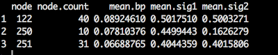
#nicely summarize the mcmc for Bill Length
output.summary.2<-ddply(.data=mcmc.data.2, .(node), node.count=length(bp), mean.bp=mean(bp),mean.sig1=mean(sig1), mean.sig2=mean(sig2), summarize)

Hmm...very strange. 250 and 251 are only tips of two sister taxa.
> this.extract<-extract.clade(tree.trim, tree.trim$edge[122])
> plot(this.extract)

Now for the Hallux:
x<-as.vector(temp$Hallux) #vector of hallux measurement traits#you have to reset the names
names(x)<-as.vector(temp$Species) #names the measurements
#use the same dated tree as before
result<-evol.rate.mcmc(tree,x,ngen=100000,control=list(sd2=2.0,sdlnr=3.0))
min_split<-minSplit(tree,result$mcmc[21:101,c("node","bp")])
mcmc<-posterior.evolrate(tree,min_split,result$mcmc[21:101,],result$tips[201:1001])
mcmc.data.2<-as.data.frame(mcmc)
#nicely summarize the mcmc for hallux
output.summary.2<-ddply(.data=mcmc.data.3, .(node), node.count=length(bp), mean.bp=mean(bp),mean.sig1=mean(sig1), mean.sig2=mean(sig2), summarize)

> this.extract<-extract.clade(tree.trim, tree.trim$edge[9])
> plot(this.extract)

> this.extract<-extract.clade(tree.trim, tree.trim$edge[29])
> plot(this.extract)

> this.extract<-extract.clade(tree.trim, tree.trim$edge[235])
> plot(this.extract)

Enough of that, let's finally look at Tail Length and see if there is anything interesting:
x<-as.vector(temp$Tail.Length) #vector of tail measurement traits#you have to reset the names
names(x)<-as.vector(temp$Species) #names the measurements
#use the same dated tree as before
result<-evol.rate.mcmc(tree,x,ngen=100000,control=list(sd2=2.0,sdlnr=3.0))
min_split<-minSplit(tree,result$mcmc[21:101,c("node","bp")])
mcmc<-posterior.evolrate(tree,min_split,result$mcmc[21:101,],result$tips[201:1001])
mcmc.data.2<-as.data.frame(mcmc)
#nicely summarize the mcmc for tail length
output.summary.4<-ddply(.data=mcmc.data.4, .(node), node.count=length(bp), mean.bp=mean(bp),mean.sig1=mean(sig1), mean.sig2=mean(sig2), summarize)

> this.extract<-extract.clade(tree.trim, tree.trim$edge[8])
> plot(this.extract)

Okay I am kind of petering out on uploading all of these. Gives me something to compare to though.
Important questions:
- Is using the extract.clade() method really capture the correct node and clade of interest?
- How are my default settings? Is this really enough time to converge?
- Reading through this helped as well:http://bodegaphylo.wikispot.org/Morphological_evolution_in_R
Next step is to start making my slides for my presentation and date random samples of trees and get feedback from adviser to make sure I am on the right track.
No comments:
Post a Comment