Implemented code from Revell, et al. (2012) in supplemental material

http://onlinelibrary.wiley.com/store/10.1111/j.1558-5646.2011.01435.x/asset/supinfo/EVO_1435_sm_suppmat.pdf?v=1&s=cb7aa4c4e828d51fd4fe1519178c9c31fd956dc6

No problems compiling the code but had to spend awhile tweaking my data set to get the names of the character data species to match the names of the nodes.

Started playing around with data to see if I could get something to orient myself. Picked a random tree from the posterior distribution of trees from Reddy/Moyle (2012) paper. Sampled randomly from my data for Wing Length and after getting all of my names to match up, I could run:

result<-evol.rate.mcmc(test.tree,x)
min_split<-minSplit(tree,result$mcmc[21:101,c("node","bp")]) 
mcmc<-posterior.evolrate(tree,min_split,result$mcmc[21:101,],result$tips[201:1001])

Error in if (where == 0 || where == "root") where <- ROOTx : 
  missing value where TRUE/FALSE needed

I ran into an error at this point and I think it is a problem that could be patched with tweaking of of the split.tree() function obtained from Revell's blog (see comment by Jessica):
http://blog.phytools.org/2011/04/updates-to-evolratemcmc-new-analysis-of.html

Seemed to fix the problem. Now onto formatting my real data set...

PCR#:	LY0002		5/22/13
	25 μL reaction
		# Tubes:	13
MasterMix	Single Tube (μL)	Total in MM (μL)
EconoTaq MM	12.5	162.5
H20	2.5	32.5
FW	3	39
RV	3	39
DNA	4	X
TOTAL:	25
FW Primer	THYF
RV Primer	THYR
Tube#	Sample
1	223167
2	582151
3	20568
4	588022
5	104610
6	110278
7	108297
8	15575
9	588479	hardly any DNA--need to extract more
10	113765	hardly any DNA--need to extract more
11	control
Program:	Omar1
Annealing Temp:	50	longer annealing time (:45)

-----------------------------------------------------------------------------------

PCR#:	LY0003		5/22/13
	25 μL reaction
		# Tubes:	13
MasterMix	Single Tube (μL)	Total in MM (μL)
EconoTaq MM	12.5	162.5
H20	2.5	32.5
FW	3	39
RV	3	39
DNA	4	X
TOTAL:	25
FW Primer	STAT5A F
RV Primer	STAT5A R
Tube#	Sample
1	223167
2	582151
3	20568
4	588022	need to extract more DNA
5	104610	need to extract more DNA
6	110278
7	108297
8	15575
9	588479	hardly any DNA--need to extract more
10	113765	hardly any DNA--need to extract more
11	control
Program:	touchdowntchup
Annealing Temp:	54

Project for Evolution 2013 meeting: predict if diversification of morphology = diversification of species.

Collected over 600 measurements from AMNH of wing length, tail length, bill length, bill width, bill depth, tarsus length, and hallux. I still need to combine the data collected from the museums in Vietnam.

First step is to impute missing data by taking the mean of that character from other measurements of the same species.

The following is the R script I wrote to do this:


#impute missing values by taking mean of all other values of of other species ofthat character 

i<-1 #set the index
species.removed<-c()
#sift through all babbler species
while (i < length(babblers$UniqueID_1)){
  #missing wing lengths; if the Wing Length is NA for that value
  if(is.na(babblers$Wing.Length[i]) == TRUE){
    #select the wing lengths of all birds which match this species with missing wing length
    wing.species.vector<-babblers$Wing.Length[which(babblers$Species[i] == babblers$Species)]
    #make a new vector without the missing value
    wing.species.filler<-wing.species.vector[which(is.na(wing.species.vector) == FALSE)]
    #calculate the mean
    wing.impute<-mean(wing.species.filler)
    #fill in missing value with the mean for that bird
    babblers$Wing.Length[i]<-wing.impute
  }
  
  #repeat the above method for all characters
  if(is.na(babblers$Tail.Length[i]) == TRUE){
    tail.species.vector<-babblers$Tail.Length[which(babblers$Species[i] == babblers$Species)]
    tail.species.filler<-tail.species.vector[which(is.na(tail.species.vector) == FALSE)]
    tail.impute<-mean(tail.species.filler)
    babblers$Tail.Length[i]<-tail.impute
  }
  
  if(is.na(babblers$Bill.Length[i]) == TRUE){
    BL.species.vector<-babblers$Bill.Length[which(babblers$Species[i] == babblers$Species)]
    BL.species.filler<-BL.species.vector[which(is.na(BL.species.vector) == FALSE)]
    BL.impute<-mean(BL.species.filler)
    babblers$Bill.Length[i]<-BL.impute
  }
  
  if(is.na(babblers$Bill.Width[i]) == TRUE){
    BW.species.vector<-babblers$Bill.Width[which(babblers$Species[i] == babblers$Species)]
    BW.species.filler<-BW.species.vector[which(is.na(BW.species.vector) == FALSE)]
    BW.impute<-mean(BW.species.filler)
    babblers$Bill.Width[i]<-BW.impute
  }
  
  if(is.na(babblers$Bill.Depth[i]) == TRUE){
    BD.species.vector<-babblers$Bill.Depth[which(babblers$Species[i] == babblers$Species)]
    BD.species.filler<-BD.species.vector[which(is.na(BD.species.vector) == FALSE)]
    BD.impute<-mean(BD.species.filler)
    babblers$Bill.Depth[i]<-BD.impute
  }
  
  if(is.na(babblers$Tarsus.Length[i]) == TRUE){
    TL.species.vector<-babblers$Tarsus.Length[which(babblers$Species[i] == babblers$Species)]
    TL.species.filler<-TL.species.vector[which(is.na(TL.species.vector) == FALSE)]
    TL.impute<-mean(BD.species.filler)
    babblers$Tarsus.Length[i]<-TL.impute
  }
  
  if(is.na(babblers$Hallux[i]) == TRUE){
    hallux.species.vector<-babblers$Hallux[which(babblers$Species[i] == babblers$Species)]
    hallux.species.filler<-hallux.species.vector[which(is.na(hallux.species.vector) == FALSE)]
    hallux.impute<-mean(hallux.species.filler)
    babblers$Hallux[i]<-hallux.impute
  }
  #if there are any values that canont be computed, remove them from the data set
  if(is.nan(babblers$Wing.Length[i]) == TRUE){
    babblers<-babblers[-i,]
    append(species.removed, babblers$UniqueID_1[i])
  }
    
  i<-i+1
}

cat("The following species were removed from the analysis:", species.removed, "\n")

I have then scaled each point to take size into account by dividing each by the geometric mean of all characters for each species. The following is the R script I wrote in order to do that:


#Size-adjust the raw data by dividing each individual by the geometric mean 
j<-1
could.not.scale<-c()
while(j<length(babblers$UniqueID_1)){
  #grab all the data of that species and put in vector
  temp<-c(babblers$Wing.Length[j], babblers$Tail.Length[j], babblers$Bill.Length[j],
          babblers$Bill.Width[j], babblers$Bill.Depth[j], babblers$Tarsus.Length[j], 
          babblers$Hallux[j])

  #calculate the geometric mean of meausrements for that species
  geo.mean<-exp(mean(log(temp)))
  
  if(is.nan(geo.mean)==FALSE){
   #divide all values for that species by the geometric mean
   geo.wing<-(babblers$Wing.Length[j])/geo.mean
   babblers$Wing.Length[j]<-geo.wing
  
   geo.tail<-babblers$Tail.Length[j]/geo.mean
   babblers$Tail.Length[j]<-geo.tail
   
   geo.BL<-babblers$Bill.Length[j]/geo.mean
   babblers$Bill.Length[j]<-geo.BL
  
   geo.BW<-babblers$Bill.Width[j]/geo.mean
   babblers$Bill.Width[j]<-geo.BW
   
   geo.BD<-babblers$Bill.Depth[j]/geo.mean
   babblers$Bill.Depth[j]<-geo.BD
   
   geo.tarsus<-babblers$Tarsus.Length[j]/geo.mean
   babblers$Tarsus.Length[j]<-geo.tarsus
  
   geo.hallux<-babblers$Hallux[j]/geo.mean
   babblers$Hallux[j]<-geo.hallux
  }
  else{
    append(could.not.scale, babblers$UniqueID_1[j])
  }
  #reset the temp
  temp<-c()
  
  #increment to next species
  j<-j+1
}

cat("The following species could not be scaled:", could.not.scale, "\n")

Now I can run a PCA on the 7 measurements to determine what holds the most variance:

#PCA for all measurements

pca.result <- prcomp(~babblers$Wing.Length + babblers$Tail.Length + babblers$Bill.Length + babblers$Bill.Width + babblers$Bill.Depth + babblers$Tarsus.Length + babblers$Hallux, data = babblers, retx = T)

Think it is better to do simple and then get more complex.
Will rerun with only the following of variables:
Annual Temp
Annual Precipitation
Diurnal Range (temperature at beginning of day and end of the day)
Seasonality

Also need to trim tiles. WAAY too big. Don't need, for example, Siberia.

Looks up paper by Mary Wiscz---distributional model of thresholding. 

Finally getting my act together and actually downloading land-use data.

Inspired where to obtain land use data from this paper:

Armenteres, et al. (2013)

Obtained land data from this website:

http://glovis.usgs.gov/

And figured out how to download land data by tile.

From LANDSAT Archives, using L7 SLC-off (2003->)list. What does SLC-off refer to?

Only downloading tiles for Vietnam, as that is what I am interested. 33 tiles in all.

The below is an excel sheet snapshot of the tiles I selected. The row and column refer to the tile. The date refers to the month and year of the tile.

How I made decisions in choosing the tile.

1) The tile must have been available for Download. For some reason, sometimes optimal tiles at some months could not be downloaded.

2) The most recent tile is preferred. Tiles were chosen from Feb 2010-Feb 2013.

3) If a downloadable, most recent tile was found, the cloud cover must have been < 10%. If no tile was found between 2010-2013 with cloud cover < 10%, the tile with the lowest cloud cover (still must be < 20%) was chosen.

Added all tiles and downloaded in full using the Bulk Download Application. Less stressful than otherwise thought. Next I will mosaic the tiles in R.

Thinking it doesn't make any sense that BIO_13 precipitation of the warmest month is most important. I also included BIO_18 precipitation of the warmest quarter.

Due to correlation values, you have to make a decision when the going gets rough. I am now going to include BIO_12 [Annual Precipitation], keep 16, get rid of 13 and 14.

R script:
#load packages
library(raster)
library(maptools)
library(dismo)
library(rJava) #also make sure to put maxent.jar into R dismo library folder

#convert to raster
altitude<-raster("/Volumes/LOLOYOHE BA/Merged_layers/alt_seasia9tile.grd")
bio2<-raster("/Volumes/LOLOYOHE BA/Merged_layers/bio2_seasia9tile.grd")

bio2<-raster("/Volumes/LOLOYOHE BA/Merged_layers/bio2_seasia9tile.grd")
bio5<-raster("/Volumes/LOLOYOHE BA/Merged_layers/bio5_seasia9tile.grd")
bio8<-raster("/Volumes/LOLOYOHE BA/Merged_layers/bio8_seasia9tile.grd")
bio12<-raster("/Volumes/LOLOYOHE BA/Merged_layers/bio12_seasia9tile.grd")
bio15<-raster("/Volumes/LOLOYOHE BA/Merged_layers/bio15_seasia9tile.grd")
bio16<-raster("/Volumes/LOLOYOHE BA/Merged_layers/bio16_seasia9tile.grd")
bio18<-raster("/Volumes/LOLOYOHE BA/Merged_layers/bio18_seasia9tile.grd")
bio19<-raster("/Volumes/LOLOYOHE BA/Merged_layers/bio19_seasia9tile.grd")


#stack the layers into one raster and name the layers within the stack

stacked.layers<-stack(altitude, bio2, bio5, bio8, bio12, bio15, bio16, bio18, bio19)
names(stacked.layers)<-c("altitude", "bio2", "bio5", "bio8", "bio12", "bio15", "bio16", "bio18", "bio19")
#remove the original rasters for space
rm(altitude, bio2, bio5, bio8, bio12, bio15, bio16, bio18, bio19)

#read locality points for first species: alcippe peracensis

peracensis.pts<-readShapePoints("/Volumes/LOLOYOHE BA/Vietnam Data/maxent_models/alcippe_peracensis_all.shp")

#run maxent for first species
maxent.peracensis<-maxent(stacked.layers, coordinates(peracensist.pts)[,1:2])

#see graph of important variables

plot(maxent.peracensis)

#see the response curves
response(maxent.peracensis)

#make raster from predictions
r.peracensis<-predict(maxent.peracensis, stacked.layers, progress = "window")


These are my models for six species showing differences between before and after changing the BIOCLIM variables to include. Notice the before is run using the maxent.jar applet rather than with R so I am still figuring out how to get all the same outputs

Alcippe peracensis Mountain fulvetta
Before:

Variable	Percent contribution	Permutation importance
bio13_seasia9tile	61.1	61.4
bio14_seasia9tile	18.1	4.3
bio15_seasia9tile	9.4	28.4
_alt_seasia9tile	7.4	0.7
_bio2_seasia9tile	3.3	1.3
bio8_seasia9tile	0.6	2
_bio5_seasia9tile	0.2	1.9

After:

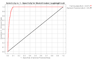
Garrulax chinensis Black-throated laughingthrush

Before:

Variable	Percent contribution	Permutation importance
bio13_seasia9tile	53.7	52.6
bio15_seasia9tile	25.7	18.2
bio14_seasia9tile	6	4.3
bio8_seasia9tile	5.5	1
_bio2_seasia9tile	4	1.3
_bio5_seasia9tile	3.9	17.4
_alt_seasia9tile	1.1	5.2

After:

Garrulax leucolophus White-crested laughingthrush

Before: 

Variable	Percent contribution	Permutation importance
bio13_seasia9tile	58.6	29.3
_bio5_seasia9tile	11.3	6.5
_alt_seasia9tile	9	18.8
_bio2_seasia9tile	7.6	13.1
bio14_seasia9tile	5.5	7.1
bio15_seasia9tile	5.1	1.5
bio8_seasia9tile	2.9	23.7

After:

Pellorneum albiventre Spot-throated babbler
Before:

Variable	Percent contribution	Permutation importance
bio13_seasia9tile	57.5	74.3
_alt_seasia9tile	17.4	1.9
bio15_seasia9tile	12.9	6.5
bio14_seasia9tile	11.8	16.9
_bio2_seasia9tile	0.2	0.5
_bio5_seasia9tile	0.1	0
bio8_seasia9tile	0	0

After:

Pomatorhinus ruficollis Streak-breasted scimitar babbler
Before:

Variable	Percent contribution	Permutation importance
bio13_seasia9tile	58.6	29.3
_bio5_seasia9tile	11.3	6.5
_alt_seasia9tile	9	18.8
_bio2_seasia9tile	7.6	13.1
bio14_seasia9tile	5.5	7.1
bio15_seasia9tile	5.1	1.5
bio8_seasia9tile	2.9	23.7

After:

Pteruthius

Should I even bother including in my analysis anymore? (No longer a babbler)

Questions to discuss:

1. Is it okay to rerun models with new set of BIOCLIM variables even if you have already run it once and just notice the first one does not seem biologically true? What if these new variables don't seem right either? Is it okay to keep trying to rerun the models?
2. What does it mean when only one variable is giving strong response?
3. Precipitation of the Wettest Month (BIO13) was removed as we had thought this didn't make much biological sense due to the way the rainy season works in SE Asia (May/June-Sept/October). We thought it made more sense if Precipitation of the Wettest Quarter were included instead (BIO 16). However, this only seemed to be important for P. ruficollis (as well as altitude). Annual precipitation seemed to be the only important variable (BIO 12) for all other species and nothing else. How can we interpret this?
4. How do I make the ROC curve in R?
5. I want to validate the model and move forward from this.

First PCR as a PhD student. Sigh.

PCR#:	LY0001
	30 μL reaction
		# Tubes:	8
MasterMix	Single Tube (μL)	Total in MM (μL)
Buffer	3	24
MgCl2	3	24
dNTPs	0.5	4
Taq	0.5	4
H20	13	104
FW	3	24
RV	3	24
DNA	4	X
FW Primer	THYF
RV Primer	THYR
Tube#	Sample
1	588460
2	580656
3	110278
4	108297
5	560781
6	control
Program:	Omar1
Annealing Temp:	50

Sample #s correlate with AMCC AMNH tissue number.